
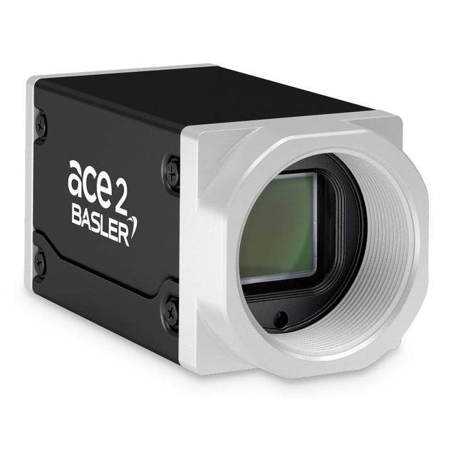
The Basler a2A2840-67g5mUV 5GigE camera with the Sony IMX487 UV CMOS sensor delivers 67 frames per second at 8.1 MP resolution.
- Rosepetal compatible
- Recommended by AIS Vision
On request
Matrix 2D cameras for full-image inspection: presence, defects, OCR/OCV and measurement.
Related searches: area scan camera, 2D industrial camera
An area scan camera captures the whole field of view in a single exposure, which makes it the default sensor for any part you can present and trigger discretely: a component on an indexing fixture, a label under a station, a board at a pick point. If your scene is a finite object rather than a continuous web or cylinder, you almost certainly want area scan, and the real work is sizing it correctly rather than choosing the category.
This guide walks the selection in the order the decisions actually depend on each other: resolution from the field of view and smallest defect, then shutter for the motion, then monochrome versus colour, and finally the interface that has to carry the resulting data rate. Get the first step right and most of the rest follows.
1,129 results
The Basler a2A2840-67g5mUV 5GigE camera with the Sony IMX487 UV CMOS sensor delivers 67 frames per second at 8.1 MP resolution.
Area scan is the correct default whenever the object can be brought to rest, or effectively frozen, in front of the camera for one exposure. That covers the overwhelming majority of discrete-part inspection: presence/absence checks, dimensional gauging on a fixtured part, surface and cosmetic defect detection, code reading, and OCR/OCV on text or date marks. Because the sensor delivers a complete 2D frame on every trigger, the imaging geometry is simple, calibration is straightforward, and you can hand the frame directly to classical tools or to a deep-learning model such as Rosepetal without reconstructing the image from lines.
The honest boundary is motion and aspect ratio. If the product is a continuous web, film, paper, textile or a rotating cylinder, or if it is so wide and so finely detailed that a single matrix frame cannot hold enough pixels across it, line scan becomes the better fit. The decision usually falls out of Step 1 below: when the pixel count a single frame would need to cover the width at your detail target becomes impractical, that is the signal to compare area scan against line scan rather than forcing a larger matrix sensor.
Two numbers drive the whole specification: the field of view (FOV) you must cover in one frame, and the size of the smallest feature or defect you must reliably detect. Write both down in millimetres, in the worst-case part orientation, including margin for part-to-part position scatter and handling jitter. The FOV is rarely just the part size; it is the part plus the wander you cannot mechanically remove.
Resolution follows directly. Divide the FOV by the smallest detail to get how many feature units span the image, then multiply by roughly 3 to 5 pixels per feature, because a one-pixel feature is indistinguishable from noise and leaves no margin for sub-pixel position, blur or contrast variation. Round up to a standard sensor format and add headroom for tolerance stack-up and imperfect optics. Resist over-specifying: every extra megapixel is more data to move, a more demanding lens and more cost, and it ripples into the interface decision later. Equally important, confirm the lens can resolve the pixel pitch you land on, because a sensor that out-resolves its lens simply wastes pixels.
Shutter type is decided by whether anything moves during exposure. A global shutter exposes every pixel at the same instant and freezes motion cleanly, which is what you want for conveyors, indexing fixtures or any part captured on the fly. A rolling shutter exposes rows sequentially; it is cheaper and often available at higher resolution for the same money, but it skews and smears moving objects and can band under pulsed lighting. As a working rule, choose global shutter for anything in motion and reserve rolling shutter for genuinely static or very slow inspections under steady, continuous light.
The choice is not isolated. Freezing fast motion means short exposures, which demand more light, usually delivered as a bright strobed source synchronised to the camera trigger. So a global-shutter decision quietly sets constraints you will revisit when you specify lighting and the camera's trigger and I/O. Most industrial area scan ranges from Basler, iRAYPLE and Omron/Sentech (STC) offer modern global-shutter CMOS sensors precisely because triggered, moving inspection is the common case.
Default to monochrome unless colour is part of the measurement. A mono sensor has no Bayer colour filter, so every pixel collects full light and full spatial detail; that means better sensitivity, better signal-to-noise in low light or short exposures, and genuinely higher effective resolution for edges, defects and text. For dimensional gauging, surface defects, presence checks and most OCR/OCV, monochrome is both cheaper to run (you control contrast with the right lighting wavelength) and easier to get a sharp, repeatable image from.
Specify colour only when the discrimination you need is fundamentally chromatic: verifying wire or label colour coding, sorting by hue, grading print or produce, or inspecting assemblies where colour is the distinguishing cue. Accept the trade-offs that come with it, the Bayer demosaicing costs you roughly a factor in true spatial resolution and some sensitivity, so a colour camera generally needs more light and more pixels to match a mono camera's defect-finding sharpness. A useful middle path for some applications is a mono camera paired with switched coloured illumination, which can isolate a feature by wavelength without paying the Bayer penalty.
Once resolution and frame rate are fixed, multiply them with bit depth to get the raw data rate the link must sustain without dropping frames, then choose the interface that exceeds that figure with comfortable margin. GigE Vision is the pragmatic default: about 1 Gbit/s over standard Ethernet, runs up to roughly 100 m, and carries power and data on one cable via PoE, which suits distributed and multi-camera cells. USB3 Vision offers more bandwidth, on the order of 350-400 MB/s, but over short 3-5 m cables, ideal for a single camera close to its PC. CoaXPress (CXP-6, CXP-12 and up) delivers multiple gigabytes per second for the highest-resolution or highest-speed area scan, at the cost of a frame grabber. Brands such as Basler, iRAYPLE, Omron/Sentech (STC) and Datalogic/Datasensing offer area scan models across these interfaces, so let the data rate and cabling pick the link rather than the badge.
Finalise the optics, lighting and physical fit last but never skip them. The lens must cover the sensor format, hit the working distance and magnification your FOV demands, and resolve finer than the pixel pitch from Step 1; for dimensional gauging where perspective error must be eliminated, a telecentric lens is often the correct, if costlier, choice. Lighting geometry, ring, dome, backlight, coaxial or low-angle dark-field, is what makes a defect visible at all and must be bright and stable enough for short exposures. Then confirm the lens mount (C-mount is common on area scan), mechanical footprint, trigger and I/O to the PLC and lighting strobe, and any ingress or temperature rating the cell needs. When the inspection itself is hard, subtle cosmetic defects or decisions that resist fixed rules, the answer is usually a deep-learning layer such as Rosepetal on correctly specified hardware, or full integration by a specialist such as AIS Vision.
A practical, application-first method for selecting an industrial camera: derive resolution from field of view and smallest detail, then match shutter, speed, interface, lens and lighting.
When to use a matrix (area scan) sensor versus a line sensor: discrete parts vs continuous web and cylindrical material, encoder sync, lighting and frame grabber needs.
How global and rolling shutters differ, why rolling shutter distorts moving objects, and when each is the right choice for industrial inspection.
We help you choose area scan cameras based on your application, FOV, working distance and environment.