Omron / Sentech ZX1 Smart Laser Sensor with Built-in Amplifier
ZX1-LD50
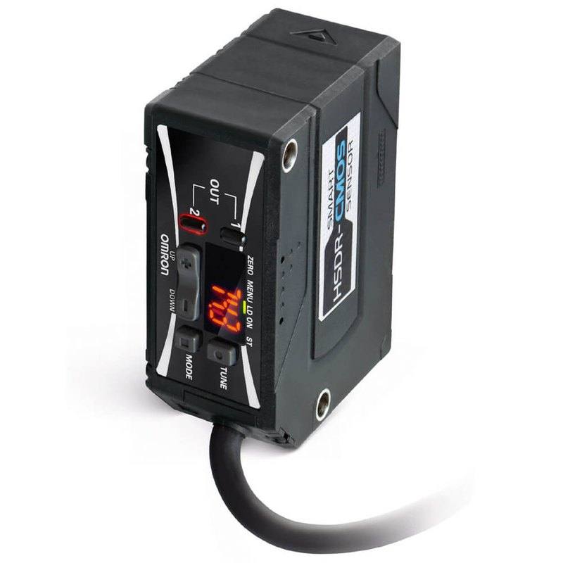
The Omron ZX1 series is a compact, self-contained laser displacement sensor using CMOS laser triangulation at 660 nm (Class 2, 1 mW max). It covers four reference distances — 50 mm (±10 mm), 100 mm (±35 mm), 300 mm (±150 mm), and 600 mm (±400 mm) — with geometrical resolutions of 2, 7, 30, and 80 µm respectively. The sensor features three selectable response modes (Super-High-Speed 1 ms, High-Speed 10 ms, Standard 100 ms), an analog current output (4–20 mA), NPN or PNP switching output, and an integrated digital display. It operates on 10–30 VDC, is rated IP67, and includes Smart Tuning for one-button setup. The "L" suffix variants use Class 1 lasers (0.24 mW) for reduced hazard ratings.
Brand
Omron / Sentech
Sensor type
Laser Displacement
Sensing method
Laser Triangulation (CMOS)
Light source
Red laser 660 nm, 1 mW max (Class 2); 0.24 mW (Class 1 'L' models)
Range / distance
50 mm ±10 mm / 100 mm ±35 mm / 300 mm ±150 mm / 600 mm ±400 mm (max far end 1,000 mm)
Response time
1 ms (Super-High-Speed), 10 ms (High-Speed), 100 ms (Standard)
Output type
Switching output NPN or PNP (30 VDC max, 100 mA max) + Analog 4–20 mA current output
The Omron ZX1 is a self-contained laser triangulation displacement sensor that integrates the optical head, CMOS receiver, amplifier, and digital display into a single compact body — eliminating the separate controller box common in earlier laser displacement designs. The sensing principle is triangulation at 660 nm (Class 2, 1 mW max; 0.24 mW on Class 1 'L' variants), which means the sensor actively projects a visible red spot onto the target and calculates distance from the angle at which the reflected beam falls on the CMOS array. This makes the ZX1 substantially less sensitive to target reflectivity variation than simple photoelectric sensors. Four reference distances are available — 50, 100, 300, and 600 mm — with measurement ranges of ±10, ±35, ±150, and ±400 mm respectively, so installers should select the model whose nominal standoff places the target comfortably mid-range, then verify the full travel of the workpiece stays within the ± window. Resolution scales with range: 2 µm at the LD50, 7 µm at the LD100, 30 µm at the LD300, and 80 µm at the LD600.
For integration, the ZX1 provides two output types simultaneously. The switching output (NPN or PNP, depending on model variant ordered — 30 VDC / 100 mA) acts as a threshold-based go/no-go trigger and connects directly to a PLC digital input without additional hardware. The analog current output (4–20 mA) carries continuous displacement data and feeds any standard analog input card or DCS channel — an advantage over voltage-output sensors in electrically noisy machine environments. Three response modes govern the internal averaging: Super-High-Speed (1 ms) is suited to fast-moving parts on conveyors or stamping presses; High-Speed (10 ms) balances noise rejection with moderate line speeds; Standard (100 ms) maximises stability for static or slow-moving measurements. The 10–30 VDC supply range covers both 12 V and 24 V plant standards without modification, and IP67 sealing (IEC 60529) permits wash-down and coolant-splash environments without additional enclosures.
Mechanically the LD50/LD100 heads measure 52.5 × 24.1 × 49 mm and weigh approximately 180 g, while the LD300/LD600 heads step up to 66 × 27.2 × 52 mm and 210 g — both small enough to mount on robot end-effectors or integrate inside machine cavities. The PBT housing with glass optical window and SUS303 stainless mounting hardware withstands moderate chemical exposure. Linearity is ±0.15% of full scale for LD50 and LD100 models, tightening the absolute displacement error to ±30 µm (LD50) or ±105 µm (LD100) across the full range — figures that make these models appropriate for genuine dimensional gauging, not just presence detection. The Smart Tuning one-button setup and the integrated display simplify commissioning: the technician can read the raw displacement value at the head without a laptop or handheld terminal, confirm the analog output span, and set thresholds on the spot.
Best for
Height or thickness gauging on a production line where parts travel at speed — the 1 ms Super-High-Speed mode ensures each part is measured within its gate window without motion blur in the displacement reading.
Robot-guided pick-and-place where a gripper-mounted LD50 or LD100 measures Z-offset to a part surface and feeds a correction vector to the robot controller via the 4–20 mA analog output.
Packaging inspection for fill-level verification, cap-present detection, or label-thickness checks where the mid-range LD100 (100 mm ± 35 mm) provides 7 µm resolution sufficient to distinguish label presence from bare substrate.
Semiconductor or electronics assembly flatness checks on PCBs, substrates, or component leads using the short-range LD50 with its 2 µm resolution and ±0.15% F.S. linearity.
Automotive and metal-stamping part presence and dimensional conformance checks in wash-down or coolant environments, where IP67 sealing and the wide 10–30 VDC supply make the sensor plug-compatible with existing machine wiring.
Selection notes
Choose the reference distance model whose nominal standoff matches your fixture geometry and verify the full displacement stroke of the target — including part-to-part variation and any vibration — stays inside the ±range for that model. The LD50 (±10 mm) is narrow; if your parts vary by more than 8 mm in height, step up to the LD100 (±35 mm).
If laser safety classification matters for your cell risk assessment, the 'L' suffix variants (Class 1, 0.24 mW) avoid the administrative controls required for Class 2 devices, at no change to measurement performance.
The 4–20 mA current output runs continuously; confirm your PLC analog input module supplies the correct loop voltage and that the cable run resistance stays within the module's compliance budget — especially for longer 10 m cable variants.
Response mode must match your line speed and acceptable noise floor. At 1 ms Super-High-Speed the internal averaging is minimal, so electrical noise on the target surface (vibration, surface texture) appears directly in the output; use High-Speed or Standard modes on stable, slow-moving targets to reduce measurement scatter.
The sensor is available in NPN or PNP switching output variants but not both simultaneously — confirm the logic polarity of your PLC digital input before ordering the NPN or PNP model, as field-swapping polarity is not possible without a replacement unit.
Specifications: General
Brand
Omron / Sentech
Sensor type
Laser Displacement
Specifications: Performance
Range / distance
50 mm ±10 mm / 100 mm ±35 mm / 300 mm ±150 mm / 600 mm ±400 mm (max far end 1,000 mm)
Response time
1 ms (Super-High-Speed), 10 ms (High-Speed), 100 ms (Standard)
These steps take an Omron Sentech (STC) camera from the box to a stable first image and on to your own application. They apply across the GigE Vision, USB3 Vision and CoaXPress STC families; the interface only changes how you cable and power the camera.
Download and install the Sentech SDK on the host PC. The package provides StViewer, the viewing and configuration software you use to bring the camera up, and StApi, the programming SDK you integrate later. Because the cameras are GenICam/GenTL-compliant, StApi also registers a GenTL producer, so any GenICam-compliant third-party vision software can discover and drive the camera as an alternative front end.
2. Cable, power and connect the camera
Connect according to the interface. GigE Vision: link to a Gigabit NIC (use PoE or the separate power input) and put the camera and host on the same subnet; for USB3 Vision use a USB 3.x port and a certified cable; for CoaXPress (STC) connect to a CoaXPress frame grabber, which also supplies Power-over-Coax. Then open StViewer and let it enumerate the camera. If a GigE camera does not appear, check the IP configuration and firewall, and on USB3 confirm the host bandwidth and driver.
3. Configure exposure, gain and white balance
Open the device in StViewer and start a live stream. Set exposure and gain for a well-exposed, low-noise image: raise exposure first and only add gain when more light or a faster shutter is not an option, keeping exposure short enough to freeze motion on global-shutter models. On colour cameras, run white balance under your actual production lighting. Adjust the lens aperture and focus on a representative target before tuning anything else.
4. Set the trigger and grab a first image
Start in free-run (continuous) acquisition to confirm a clean, stable image. For inline inspection switch to hardware or software triggering: select the trigger source, set the active edge and any delay, and wire the strobe or illumination to the camera's I/O so lighting fires with each exposure. Acquire and save a frame in StViewer; this saved image is your reference for the SDK stage and for downstream inspection.
5. Move to the StApi SDK (or any GenICam software)
Once the image is stable, reproduce the same settings in code. Use StApi to open the device, apply the GenICam features you validated in StViewer (exposure, gain, trigger, pixel format) and grab frames into your application via the bundled C++, C, C#/.NET or Python interfaces; the included samples are the fastest starting point. Prefer a different stack? The same GenICam/GenTL camera works with third-party vision libraries. With a reliable feed, you can route it into a deep-learning inspection such as Rosepetal for AI-based defect detection.
Frequently asked questions
Resolution depends on the model: 2 µm for the LD50, 7 µm for the LD100, 30 µm for the LD300, and 80 µm for the LD600. Note that resolution is the minimum detectable step; absolute accuracy is governed by linearity, which is ±0.15% of full scale for LD50/LD100 — equating to ±30 µm and ±105 µm respectively across the full measurement range.
Yes. The sensor is rated IP67 per IEC 60529, meaning it is protected against temporary immersion up to 1 m. The PBT housing and glass optical window are suitable for coolant splash and mild chemical environments. The optical window must remain clean for accurate readings; periodic cleaning is recommended in high-contamination environments.
No. The ZX1 integrates the amplifier, display, and output conditioning into the sensor head. It connects directly to a 10–30 VDC supply and provides both a switching output (NPN or PNP depending on model ordered) and a 4–20 mA analog output without any additional controller box.
The fastest mode is Super-High-Speed at 1 ms response time. Whether that is fast enough depends on part length and conveyor speed — at 1 m/s a 1 ms window corresponds to 1 mm of travel. For applications requiring precise measurement within a tight gate window, ensure the encoder or trigger signal activates the measurement while the target is fully within the sensing spot.
Pre-wired cables come in 2 m, 5 m, and 10 m lengths and are the simplest option for fixed installations. The 0.5 m connector pigtail suits applications where the sensor is replaced frequently or installed in a cable-chain, since the field cable can remain in place and only the sensor head is swapped. Confirm cable run resistance is within your analog input module's compliance window for the 4–20 mA output.